Recommended articles:
-

-
Global Energy Interconnection
Volume 8, Issue 4, Aug 2025, Pages 668-684
New strategy for fault detection and classification in wind turbines based on doubly-fed induction generators☆
Abstract
Abstract
0 Introduction
1) Motivation and incitement
Environmental preservation and sustainable development of energy resources are currently at the center of global concerns [1].As a result, alternatives to increased exploitation of fossil resources increasingly consistof resorting to the sustainable and efficient developmentof renewable energy sources such as wind energy.The latter is gaining momentum thanks in particular to its main advantages in terms of increased energy production,guaranteed long life and flexibility in terms of the energy mix and the integration of wind systems into the electricity grid[1].Furthermore, we can say that the concept of sustainability in the sense of wind systems consists not only in meeting energy and economic needs,but also in preserving today’s environment, without compromising the capacities, assets and challenges of this clean energy for future generations[2].However,it is not at all easy to find a good compromise between ecological balance, and guaranteed long life for wind turbines on the one hand, and facilitat e the integration of wind turbines into an electrical network onthe other hand.The main reason is that the exploitation ofwind energy is faced with the resolution of very complex major problems that fall within the fields of high-level research.
Nomenclature N Artificial neural network RC Active disturbance rejection control N Convolutional neural network OS Dedicated observer structure LPC, DLIM and DLIP Defects related to the setpoint, the model and the parameters DS Fault linked to set point disturbances E Extended Kalman Filter T Fast Fourier Transform RC High resistance connection C International Electrotechnical Commission Diagnostic system T Linear fractional transformation I Linear matrix inequality CSA Machine current signature analysis ANFIS Multiple output neurofuzzy inference C Rotor side converter Takagi-Sugeno Transmission Lines KF Unscented Kalman Filter Artificial intelligence AN AD CN DD F L FK FF H IE Ξ LF LM MMR S TS TL U AI βDΔ 1 FL FL FS GHI G χ2 LP LM MℕRT C θj VM∊R* Adjustment factor of the hyperbolic tangent function FIG Doubly-fed induction generators, δ Transfer matrix for model and parameter uncertainties MU Fault linked to model uncertainties PU Fault linked to parameter uncertainties A French Standardization Association OS Generalized observer structure inf Infinty Horizon BT Insulated gate bipolar transistor Chi-square V Linear Parameter Varying Leveuberg-Marquardt PPT Maximum Power Point Tracker Set of natural numbers Set of real numbers SC Thyristor-controlled series capacitor Activation threshold of neurons D Variational mode decomposition
We can therefore distinguish two major groups of challenges related to the exploitation of wind energy.The first group of problems concerns [3-5]:
The search for new sustainable materials those are more suitable for the design and manufacture of innovative and ecological wind turbines;
The planning and location of sustainable wind farms onshore and offshore;
The greener energy mix;
The life cycle analysis of wind systems;
Visual pollution and noise pollution from wind turbines;
Handling, assembly and maintenance of wind infrastructure etc.
This first group of problems can directly or indirectly influence the quantity and quality of wind energy produced [3].Therefore, the second category of problems related to the production of quality and quantity of wind energy concerns [1,3-5]:
The risks of untimely disconnection of the wind turbine from the grid;
The increase in the harmony rate;
Voltage dips flicker;
Maximization and storage of the energy produced;
Decoupling and control of active and reactive power ofwind systems;
The energy and/or economic profitability of wind turbine control and diagnostic strategies;
Excessive temperature rise in the DFIG coils and in the static converters of the power electronics of the wind system, etc.
Indeed, in practice the complexity of problems related towind turbines intensifies with the increase in requirements in terms of research for a better quantity and quality ofthe energy produced on the one hand.And on the other hand, the increase in constraints concerns the choice of control techniques, maintenance strategies and the choice ofmodels used for optimal exploitation of wind energy.Therefore, our motivation in this work aims to guarantee automated wind systems good availability or operational safety.To do this, we generally use diagnostic methods that mainly refer to the concept of conditional preventive maintenance, based on continuous monitoring of the system considered.Unlike corrective maintenance, whose action occurs after the system considered has suffered a failure or breakdown.The preventive maintenance approach requires a diagnostic system beforehand, in order to allow early detection of malfunction deviations from the normal operation of a system.This latter approach will retain our attention throughout this manuscript, in order to contribute to the proposal of a robust and optimal diagnostic system allowing us to better respond to the major challenges linked to the production ofwind energy in quantity and quality.
2) Literature review
In order to respond effectively and efficiently to the resolution of problems related to the quality of energy produced by wind systems.Most researchers are dedicated to the use and development of optimal control strategies and robust diagnostic systems.Although it is almost diffi-cult to dissociate optimal control from robust diagnostics in complex systems, we will nevertheless be interestedin reviewing the work on the development of robust diagnostic systems.In general, there are two main familiesof methods in diagnostic systems, the quantitative diagnostic family which uses methods based on mathematical models of systems and/or signals.While,the qualitative diagnostic family uses methods based on artificial intelligence(AI)or based on numerical calculation optimization algorithms.Indeed, these two families are not disjoint; the joint use of qualitative and quantitative methods offers a good exploitation of all the deep or available knowledgeon the behavior of a system or signal studied.Therefore, the state of the art on the most recent works that we present in this manuscript is split into two large groups, namely,the first group for diagnostic systems based on quantitative approaches, and the second group for so-called hybrid approaches which combine qualitative and quantitative methods.
a) First group of works based on quantitative approaches
Mohamed-Amine et al.[6], propose a diagnostic method based on an augmented state and disturbance observer combined with an X2 (chi-square) test.This approach will be experimentally verified on a 15 KW test bench, in order to ensure fault detection on IGBTs, rotor and stator current sensors, as well as failures on stator voltage sensors.However, this method can mainlybe improved,with regard to complexity,increased use of sensors and actuators, accuracy in identifying and localizing the nature of faults, cost, etc.Abdelwahab et al.[5], propose a review of different methods for detecting internal electrical faults in the DFIG for wind turbines.The authors review the models for accurate fault analysis and estimation, as follows:
Robust and inexpensive methods based on stator current,the main limitation of which is high sensitivity to anomalies;
Wavelet analysis methods for multi-resolution detection,with the main drawback of low sensitivity to minor defects;
High-precision methods based on equivalent magnetic circuits, but very strongly affected by parametric variations of the machine;
Fast methods based on Fourier analysis, which are very affected by speed fluctuations;
Precision methods based on combinations of machine current signature analysis(MCSA)are also affected by changes in torque or speed;
Simplistic methods based on vibrations have limitations in terms of context and implementation;
High-precision methods based on the study of flows have drawbacks in terms of reliability, cost and complexity.
Overall, these methods require improvements in terms of sensitivity to minor or major faults on the one hand;but also in terms of cost, reliability and complexityof implementation, particularly when it will be necessary to consider and federate all these methods at once for a more complete wind turbine diagnostic system.
Yosra Sayhi et al.[7], uses a test bench based on the dedicated observer structure (DOS) and the generalized observer structure (GOS), to ensure the detection and localization of intermittent faults of sensors and interwound short circuit of the DFIG.This work, whichis too specific,will be even more complex when it will be necessary to carry out other notifications and manipulationof tests, in order to take into account other types of defects.
Wei Ding et al.[8] will focus solely on the diagnosisof stator resistance unbalance faults.The approach they proposed is based on banks of shunt capacitors, on an artificial neutral point and on the assumption of excellent control performance.Therefore, even if the approach could prove to be more complex,it requires an application feasibility study by evaluating the impact of optimal controllers on the one hand.On the other hand,it is important to associate with this approach, a classification method making it possible to diagnose high resistance connection faults(HRC) in the stator and rotor windings of the DFIG.
I Idrissi et al.[9], propose a diagnostic approach based on the Kalman filter of the Linear Parameter Varying(LPV) type which integrates the parametric variationsof the DFIG.Additionally, the nonlinear variantsof Extended Kalman Filter (FKE) and Unscented Kalman Filter (UKF) are used for disturbances and noise.Although effective, this approach requires improvement in terms of the use of a reduced number of sensors and actuators which can drown out certain noises,and complicate the identification, precision and localization of other types of DFIG faults.
b) Second group of works based on hybrid quantitative and qualitative approaches
Ikram Aissaoui et al.[10] propose a fault-tolerant control strategy for current sensors on the DFIG of the wind turbine.The approach is based on the optimized active disturbance rejection control(ADRC).The genetic algorithm isassociated with the detection, identification, isolation and reconfiguration of current sensor signals after a failure.This very targeted approach needs to be improved byusing a more robust diagnostic system that considers other types of faults to improve the localization and nature ofthe faults.
Hadjira Bouazza et al.[11],propose the fuzzy inference approach and ANFIS for the detection of faults in the switches of the rotor side converter(RSC)of the DFIG of wind power.This approach is based on prior determination ofthe detection threshold based on the average values of the three-phase currents of the rotor.Although the approach is apparently simple, effective and rapid in detection, it can however be criticized for the validation or practical feasibility,detection accuracy,integration,localization and identification of other types of DFIG defects.
Nasreddine Labe`d et al.[12], propose a strategy that involves not only the Fast Fourier Transform(FFT)algorithm to extract frequency characteristic parameters, but also using ANFIS adaptive neuro-fuzzy inference to detect and Automatically classify DFIG rotor and stator faults.Although this method demonstrates effectiveness and reliability, it is nevertheless necessary to explore the strengths ofthis approach more extensively, and by comparing it to other diagnostic methods based on ANN and Fuzzy logic for DFIG.
Esvan-Je´sus Pe´rez-Pe´rez et al.[13], propose a hybrid approach for fault detection and isolation on a 5 MW wind turbine.The approach consists of an ANFIS that identifies the dynamic model of the wind turbine and results in a quasi-linear polytopic ensemble with variable parameter (qLPV).Fault detection is performed from a residual generator consisting of qLPV zonotic observers.Inaddition, the training of the ANFIS fuzzy neural network uses only healthy data without defects.The robustness and satisfactory performance of the approach is tested with the perturbations related to the aerodynamic load and the measurement noise.Furthermore, Esvan-Je´sus Pe´rez-Pe´rez et al.[14] propose another 5 MW wind turbine fault diagnosis system consisting of a zonotopic state estimator based on Takagi-Sugeno (TS) models with parametric uncertainty association using multiple output neurofuzzy inference (MANFIS).The fault detection and isolation via a fault signal matrix is based on the TS zonotopic observer.The linear matrix inequality(LMI)ensemble with Hinf ensures the adjustment of the observer parameters by taking into account the model uncertainty.The proposed approach, unlike the one presented in [13],offers an improvement in terms of operability,fault identification, uncertainty estimation and learning time.
Along the same lines, Esvan-Je´sus Pe´rez-Pe´rez et al.[15], develop another fault diagnosis approach for the 5MW wind turbine, based on the use of a set of TS interval observers to detect and isolate sensor faults.The ANFIS model allows obtaining a polytopic linear representation and the membership models to interpolate the linear models of the convex TS.The main advantage ofthe approach [15] is to generate confidence intervals,inorder to prevent modeling errors.
Sauvik Biwas et al.[16] proposes a distance relay algorithm for the protection of transmission lines that are connected to the wind farm based on DFIG.The proposed algorithm extracts useful features from the line current signals, using a single-pole filtering technique to generate red-green-blue images of the ANN classifier, to improve fault detection and classification.The approach is validated by real-time numerical simulation using fault-free and fault-free data from the two-bus and nine-bus test power systems for thyristor-controlled series capacitor(TCSC) wind farms with DFIG.The performance of the approach is 100% for detection accuracy and about 99.50% for fault classification accuracy.Sauvik Biwas etal.[17], further proposes an intelligent distance relay scheme for fault detection and classification in transmission lines (TL) which are connected to the output signals ofthe wind generator with DFIG.The proposed approach, uses a variational mode decomposition(VMD) to extract in real time, the characteristics of the line current including the extraction of the frequency components of the faulted current and in order to distinguish internal faults from external faults.The quantities extracted by the VMD pass through a Wiener filter to generate the gray level images which will be used by the deep convolutional neural network (CNN) classifier.The effectiveness of the proposed algorithm is evaluated by realtime simulation on a two-bus system using 12,000 fault cases and 120 non-fault cases and to compare them at least with 5 different approaches.The approach shows satisfactory performance with a fault detection time of 10 ms,high fault detection and classification accuracy of 100% and 99.86% respectively.
Sauvik Biwas et al.[18] further propose a relay algorithm based on the use of sign of the half-cycle superimposed positive sequence current for fault detection on thyristor controlled series capacitor (TCSC) compensated(TL) wind farms with DFIG.An empirical compensation-assisted random forest classifier provides fault classification.While a modified impedance approach provides fault localization.The performance of the proposed algorithm is evaluated on 6750 fault cases and many transient cases without faults generated on a test system in Matlab Simulink.The approach presents 8 ms performance in detection and classification, with accuracies of 100% for detection, 99.12% for localization and 99.95%for fault classification accuracy.Sauvik Biwas et al.[19]propose another smart relay scheme to protect transmission lines (TL) connecting wind farms based on DFIG.The proposed scheme for line fault detection and identification is based on the use of α-aerial signs superimposed onthe current measured at the TL end at the static synchronous compensator (STATCOM).The measured currents are then extracted at the relay end usinga double-time transform (TT) to be used by a decision tre e classifier to classify the faults.A technique based on the use of positive waves of α and β aerial currents is used to estimate the faults.The effectiveness of the approach is evaluated with 6000 fault cases and many transient cases without faults simulated from a test system in Matlab Simulink.Unlike the works [16-18], the proposed approach requires less inputs, low computational load,reduced implementation difficulties.The detection and classification are of the order of 8 ms, the detection accuracy is 100%, the location accuracy is 99.18% and the defect classification accuracy is about 99.96%.
Although the performances of the approaches proposed in the second group of works are satisfactory for the diagnostics of faults on the current sensors of the machine, on the switches of the rotor-side converters, on the current frequencies of the DFIG, on the wind turbine and on the transmission lines of wind farms.However, the proposed hybrid approaches still encounter some limitations and challenges summarized as follows:
The proposed approaches focus on the diagnosis ofa single element of the wind system at a time, without taking into account the global analysis of the wind system, in particular the interactions between turbine,machine, converters and network.
Giventhecomplexityofthedevelopmentoftheproposed approaches by simulation, experimental feasibility assessmentsarenecessaryfortheircompletevalidations.The fact that the qualitative approaches used do not necessarily use mathematical models of the systems;can lead to a deprivation in the acquisition of knowledge and analysis of the global and intrinsic behavior of the systems studied.Therefore, the identification and localization of isolated faults are subject to risks of ambiguities.
The difficulty related to the collection of healthy data or the use of erroneous data for the training ofAI algorithms can influence the effectiveness of the diagnostic results in terms of high time and risk of error.In addition, the manipulation or use by these approaches of a large number of data, sensors and actuators necessarily leads to an overconsumptionof energy, an increase in the learning time, and an increase in maintenance difficulties and costs.
Unlike mathematical approaches,the training data for qualitative approaches are not easily generalizable to allwind systems, because theuncertainties vary from one manufacturer to another.
3) Contribution and paper organization
The main objective of this work is to propose a robust and more complete diagnostic system for the detection,localization and classification of wind system faults based on the DFIG.To do this,a new hybrid approach is envisaged as follows:
The structured modeling of the DFIG based on the Linear Fractional Transformation (LFT) representation has the role of associating the observed output states with the sensors and/or actuators in order to facilitate the identification, detection and localization of faults due to the uncertainties of the parameter s and the model of the system studied.In addition, the LFT structure of the DFIG will allow the identification of impacts related to faults coming from the instructions or interactions between the different elements of the wind system studied.Unlike the approaches mentioned in the literature, the DFIG LFT will facilitate the implementation of a robust and more complete diagnostic system based on the structured identification and localization of possible uncertainty and setpoint faults arising from the interactions between turbine, machine, converters and network of a wind system.
The use of the parity space or analytical redundancy approach aims at the detection,identification and effi-cient localization of faults on the outputs of the observed states of the system.Unlike observation models such as the Kalman filter for example,the parity space approach offers the advantage of using fewer sensors and no control actuators.The robust hybrid diagnostic proposed based on the analytical redundancy approach associated with the ANN structure also consists in dedicating the ANN structure to evaluate or locate and classify only the hidden faultsor those that were indistinguishable from the quantitative method called parity space.This hybridization approach envisaged offers the possibilities of reducing the number of data and learning times,of reducing the number of sensors and actuators required and of also reducing the overconsumption of energy.Consequently, this will allow the reduction of the difficulties of maintenance of the system and the reduction of the complexity and the cost of the proposed diagnostic system.
The classification of the faults will consist in associating the outputs of the observed states of the models by parity space with the ANN,in order to better structure the monitoring of the diagnosis and to allow an optimal intervention during the maintenance of the wind system based on the DFIG.
This work is organized as follows:
The methodological part will consist in demonstrating in detail the proposed diagnostic approach such as,the LFT structured modeling of the DFIG; the detection,identification, localization and classification of the observed faults of the diagnostic system based on the static redundancy approach associated with the RNA.
The results and discussion part is devoted to the analysis, interpretation and validation of the proposed diagnostic results.
The last part is devoted to the conclusion of the presented work.
1Methodology
To situate the context of the robust diagnostic system envisaged, we will rely on the position and the fundamental roles that the DFIG plays in a wind system as represented by Fig.1.The latter places the DFIG as the central element of the wind system, whose main function isto transform mechanical energy from the wind into electrical energy transmitted to the network.The Maximum Power Point Tracker (MPPT) controller of the wind turbine will allow maximum exploitation of wind energy and regulation of the mechanical energy transmitted to the DFIG.While, the other controllers associated with the RSC and GSC will ensure the energy exchanges between the generator rotor and the electrical network.Then, by magnetic induction, energy exchanges will be guaranteed between the DFIG stator and network.Consequently, the need for a robust diagnostic system based on the equivalent DFIG model is essential, in order to guarantee good operational safety and better maintenance of wind energy systems.
1.1 Generalized model of DFIG
The envisaged diagnostic system will exploit the equivalent dynamic model of the DFIG defined in the Park’s(d,q)framework as follows [1]:

where, Usd, Usq and Urd, Urq are respectively the expressions of stator and rotor voltages in reference (d, q);
Msr and Mrs:the mutual inductances between the stator and rotor windings are generally considered identical by the relationship; With, Msr = Mrs = M;
rr, rs: The resistors of the rotor and stator windings;
Lr, Ls: The inductances of the rotor and stator;
ωos and ωr:The angular speeds of rotation from field to stator and rotor respectively;
isd,isq and ird,irq:The currents flowing to the stator and rotor respectively in the d axis and q axis system.
1.2 Principle of structured representation by LFT
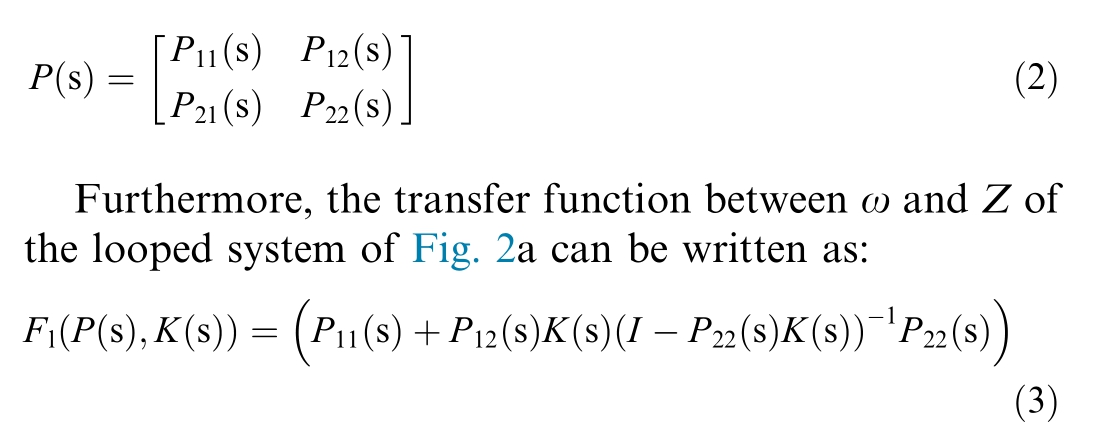
In principle, the LFT representation is a structured modeling of a multi-variable system which includes the reference model and the uncertainty models.Clearly,a representation by LFT consists of determining the augmented model P(s) of a multi-variable system, either for the synthesis of a control law in Fig.2a,or for a case of synthesis of’a robust diagnostic system of Fig.2b.Hence, the description of Fig.2 such as:
K(s)and Ξ is respectively the corrector and the diagnosticsystem sought;
P(s), the controlled process or general process of the system;
ω, Gathers the inputs considered such as reference signals, disturbances and noise.
U, the process control vector;
Z, the vector of outputs or signals chosen to characterizethe proper functioning of the controlled process P(s);
Y, the vector of outputs or measurements of the process;
X, the state vector represents the internal variables of the process.
The general process is also called augmented matrix,and its partitioned representation is given as follows:
1.3 LFT structured representation of the DFIG
The formulation of the LFT representation applied to the DFIG for the diagnosis of a wind energy system,and including the mixed uncertainties (model and parameter uncertainties) is given by the structuring of Fig.3.Indeed, a complex and multivariable system like the wind power DFIG must take into account the uncertainties of parameters and/or models.In Fig.3, model uncertainty(Wm), represents high-frequency dynamics as a single block transfer matrix (Δ1), which can be summed or multiplied by the process reference model.Whereas,parameter uncertainties in the form of matrix structuring in a block(δ), represent parametric variations of the dynamics and/orelementary coefficients of the process.
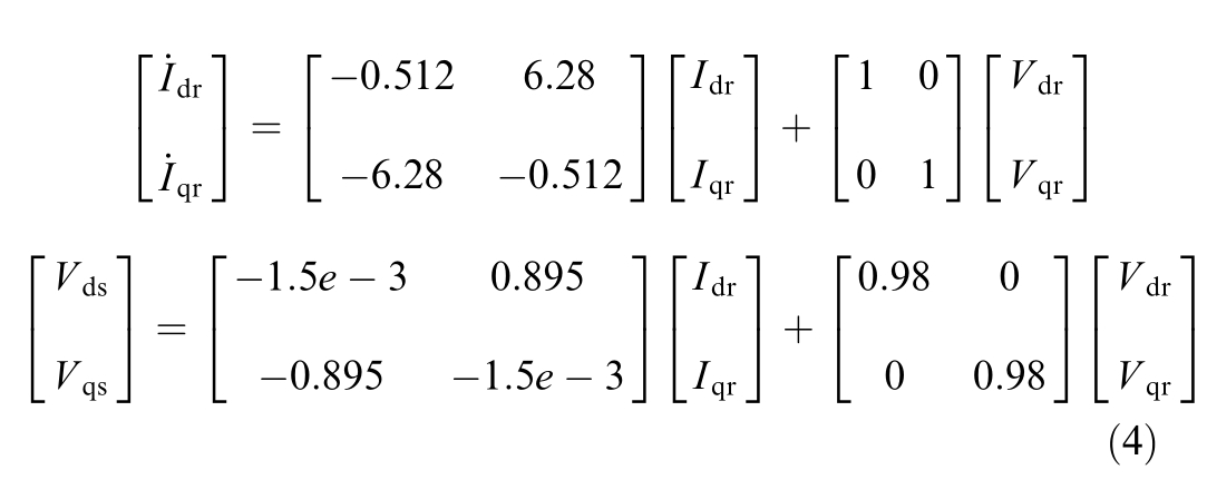
By rearranging (1) and using the DFIG parameter values in Table A1 in the appendix, we arrive at the expression of the matrix state equations of the DFIG dynamic reference model, as follows:

Fig.1.Wind system integrated into an electricity network based on DFIG.
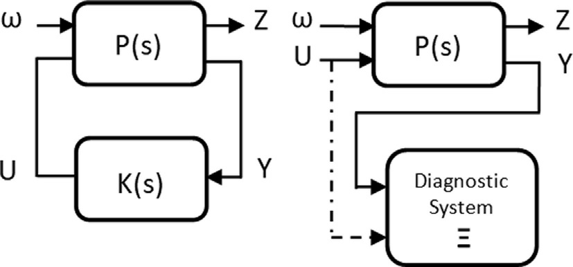
Fig.2.LFT representation for control(a)and diagnostic(b)summaries.
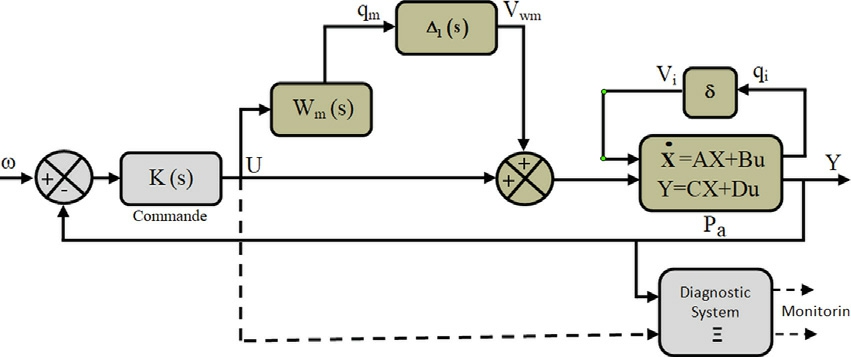
Fig.3.LFT structuring of mixed uncertainties including control and diagnosis.
1.3.1 Choice of parameter uncertainty in the DFIG
In practice, whatever the influences of faults, the parameters of a system can be modified at any time bya control law, in order to guarantee the stability of the controlled system [4].As part of the dynamics of a wind energy system and thanks to the control laws, the DFIG can operate in its four-quadrant mode around the synchronism point g (slip).Knowing that the slip g is directly linked to the mutual inductance M at the stator level,we can directly target the uncertainty parameters linked to the slip in (4), such as [1]: 6.28 = ωsg and 0.895 = Mωsg;where ωs the stator pulsation.Therefore, we can consider that the sliding can belong to a speed range of ±30%,hence g ∊[0.014 0.026] with g = 0.02.We will writeg according to a real normalized uncertainty noted |δ| <1 as follows:
With, g0 = (0.014 + 0.026)/2 and g1 = (0.026 + 0.014)/2
1.3.2Choice of model uncertainty Wm and augmented matrix of DFIG
In practice, the modeling errors of a DFIG fundame ntally constitute the source of model uncertainties.Therefore, and according to the principle of vector control,we can admit that the transfer function of the nominal model G(s) of the DFIG is of the 1st order.Then, let us also assume that the applied command comes from a fast and dynamic 1st order actuator [1].We can then write the model G¸(s) of the system, including the uncertainties which come from the unmodeled dynamics in the following form:
With, Tm, the time constant of the actuator.(We chose Tm = 0.0001).
The multiplicative model uncertainty on the represent ation of Fig.3 is given by the following expression [1]:


By rearranging (5) and (7) in (4), we obtain the following LFT augmented system of the DFIG:
![]()
1.4 Summary of the parity space approach for the DFIG diagnostic system
According to the definitions of the French Standardization Association (FSA) and the International Electrotechnical Commission (IEC), diagnosis is defined as the identification of the probable cause of failures using logical reasoning based on a set of information from an inspection, control or test [20].Indeed, we mainly encounter two types of diagnostic approaches, namely the quantitative approach which does not necessarily use the laws of physics, and the qualitative approach which uses mathematical models for detection and analysis locating faults ina system or signals.The quantitative approach which isthe subject of our diagnostic study generally follows a quantitative monitoring representation described by the steps in Fig.4.The process to be monitored which receives the command U(t) as input, and delivers a measured output Y(t), is exposed to the noise sensitivities of the unknown inputs d(t), and to the influences of faults f(t)that we wish to detect.The residual generation step uses amathematical model to determine symptoms or residuals, based on control actuator observations of U(t), and/orsensor measurements of Y(t).Whereas, the residual evaluation step consists not only of detecting faults from non-zero residuals, but also of locating or identifying faults based on a fault signature,or based on the classification of defaults.
The main objective of a fault classification is to implement a good protocol for precise location or identification offaults (the sources, causes and/or nature of faults).In addition, fault classification consists of defining a good monitoring protocol for a diagnostic process, with the aim of facilitating decision-making and the operationalization of the maintenance process of a system.Consequently, the last step in Fig.4 is simply dedicated to monitoring and/or making decisions either for setpoint orcommand changes,or for voluntary stops, or for emergency stops of a process [21].
1.4.1 Principle of static redundancy of the parity space approach
In general, there are three large families of approaches used to determine a diagnostic system, namely the parity space approach, the observer approach and the family of parameter estimators [21-23].In the parity space family,wefind the static redundancy approach and the dynamic redundancy approach for the case of discrete systems.In principle, the choice of an approach can be guided not only by the search for the best performance or solutions,but also by the subjective ability of a researcher to be able topropose sustainable and effective solutions to given problems.Unlike other approaches, static redundancy offers great advantages in terms of reducing the complexity ofthe envisaged diagnostic system and facilitating the optimal implementation of diagnostic systems associated with the ANN.In addition, static redundancy allows the use of a reduced number of sensors and actuators facilitates practical feasibility and ensures operation in stationary mode.The principle of static redundancy consists of searching for existing relationships between sensor measurements and the faults associated with them.To do this,the mathematical model of the diagnostic system envisaged can be written as follows [23]:
where p and n, represents the dimension of a matrix;nating x(t)in(9),depending on whether the matrix C must
y(t) ∊Rp is the vector of measurements;
C ∊Rn*p is the observation matrix;
X(t) ∊Rn is the state vector;
f(t) ∊Rp is the fault vector linked to the sensors.
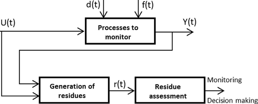
Fig.4.Representation of a quantitative monitoring process.
The redundancy expressions are determined by elimibe of full column rank and whether the number of measurements on y(t) must be greater than the dimensionof x(t).From then on, it will be possible to determinea matrix V of such that we have VC=0.To do this,we multiply (9) by V, and we obtain the generalized equationof the residual generator, also called the vector of the parity space, given by the following expression [23,24]:
where,Vi(t),is the column vector number(i)of the projection matrix V in parity space; so that in the absence ofa fault the residue is zero, and in the presence of the fault fi(t) the residue r(t) is rather oriented in the directionVi(t) of the defective sensor.
Furthermore, the most popular approach to determining the parity matrix V consists first of considering that we are in the absence of the defect.This allows us to rearrange (9) and rewrite it as follows:
where, y’ (t) = [yn (t) yp-n (t)] T and C’= [Cn Cp-n] T.
With,Cn is an invertible square matrix obtained from n first row of C.Whereas, Cp-n is a second matrix obtaine d from the remaining rows of C.We can then write the following relation:
Eq.(12)allowed us to chase away the unknown x’(t),in order to verify the consistency of the measurement,and to deduce the following redundancy equation:

where,V’=[-Cp-nCn 1 Ip-n]is the parity matrix orthogonal to C’, and satisfying the condition V’C’ = 0.We can the n deduce the fault signature table from (13).
1.4.2 Summary of the static redundancy approach applied to the robust diagnosis of DFIG
Considering the conditions for formulating(11),we can by analogy extract and rearrange the observation matrix of(8),in order to obtain the equation of the robust DFIG diagnostic system, as follows:


With, C1 the invertible square matrix and belonging to the first row of C’.And, C2 is the second matrix obtained from the remaining rows of C’.The measured output (y’)will house four measurement sensors.
The eliminationofx’in(14),allows ustodetermine the parity matrix![]() such that the expression V’C’ = 0 is true.Thus, we obtain the calculation of the parity matrix orthogonal to C’, as follows:
such that the expression V’C’ = 0 is true.Thus, we obtain the calculation of the parity matrix orthogonal to C’, as follows:
From (15), we can easily deduce the following redundancy matrix or residue generator expression:

Eq.(16) makes it possible to construct the fault signature table presented in Table 1.The latter means, the residue r1 is sensitive to the faults fvds,fvqs and fqi.While,r2is sensitive to the fault fqm.As r1 is sensitive to faults fvds,fv qs and fqi, and if faults occur at the same time and with di fferent amplitudes, this can make it difficult to visualize similar faults or faults with very low amplitudes.To allow better identification and good localization of similar defects and/or very low amplitudes, we are considering an automatic classification (precise and distinct) of these types of defects based on ANN.
1.5 Summary of the ANN-based defect classifier
The synthesis of fault classification first consistsof defining a protocol for precise location or identification of faults based on the analysis of the operation of the diagnostic system established based on the static redundancy approach.Then, from the analysis of the results of the diagnostic system, we will implement and associate an ANN structure to ensure the automatic and structured classification of similar or non-discernible defects and hidden defects.
1.5.1 Principle of a formal neuron
Formal neuron modeling is a mathematical representation in the form of a threshold adder,multiple inputs anda single output,as shown in Fig.5.The latter is likened toa biological neuron thanks to the following two main [25]:

where, Si (k), Sj (k) and Wij (k) are respectively the ith input,the output of the neuron and the weight of the connection between neuron i and neuron j.tion threshold of the neurons.
f(.) is the activation function of the neuron and can be stepped, sign, or non-linear, etc.
A neural network is an interconnection of formal neurons between them, with the aim of carrying out prediction, modeling, control or diagnostic functions, etc.In addition, a neural network mainly obeys open loop architecture or either closed loop architecture.
1.6 Implementation of ANN for classification of indistinguishable faults in diagnostic system
In practice,there is not yet a fixed method to determine orto choose a neural architecture for classifying defects in adiagnostic system.Therefore, we propose a qualitative method based on ANN to evaluate or locate and classify only the hidden defects or the defects that were indistinguishable from the quantitative method called parity space.To achieve this,the neural network learning method weadopt in this work is carried out in three main stages:
Zj (k) is the input function and θj is the bias or activa-
The stage dedicated to collecting training data;
The stage concerning the selection of the configuration and training of the proposed neural network;
The stage focusing on validating the implemented neural network.
1.6.1 Training data collection stage
To collect data relating to the signature of hidden or indistinguishable defects, we use data extracted from the signals identified on the inputs and on one output of the residual generator obtained based on the parity space model.From then on, we can collect four samples of 1278 data points on each of the residual generator inputs toconstitute the data for four inputs of the proposed ANN.Then, we also collect a sample of 1278 data from the output of the residual generator for the training output ofthe ANN.
Table 1 Defect signature table.

fvd fvq fqi fqm r1 1 1 1 0 r2 0 0 0 1 s s
1.6.2 ANN structure configuration and training step
The implementation of the indistinguishable fault model we adopt is based on supervised learning defined inthe neural structure of the Matlab ‘‘Neural Network ToolBox” utility [25,26].Once in the utility, we select the‘‘Fitting Tool” assistance,which allows us to take the collected data and input it into the training database to define the ANN structure and its inputs and outputs,as shown in Fig.6.
Clearly, the defect model implemented on the ANN structure of Fig.6 has four inputs and one output, the weights and the activation thresholds of the neurons are respectively noted (w) and (b).Fig.6 consists of a total of11 neurons, including 10 neurons in the first hidden layer and 1 neuron located in the output layer of the structure.The use in the first hidden layer of the hyperbolic tangent activation function that varies in the interval 1 and 1,aims to take into account and better evaluate the highly nonlinear behavior of the ANN input quantities.The expression of the hyperbolic tangent activation function can be written as follows:
where, Zj (k) the input function of the neuron is given by(17).
β∊R*, is the factor or parameter for adjusting the activation function f,in order to avoid the problem of saturation of the said function.
Then,the signals that will be processed in this first hidden layer can be normally directed to the outputs of the ANN via an activation function of the output layer of the linear type whose polynomial function can be written asfollows:
With,ai ∊R,the coefficients of the polynomial of degree(i), and n ∊ℕ.
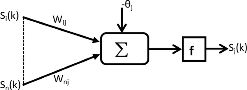
Fig.5.Representation of the neural model.
The training of the utility’s ANN structure depends on the amount of input and output data we insert into its database.In our specific case, the assistance makes an optimal choice for our data, dedicating 70% of each sample of our input-output data to training,then 15%of each sample for testing and the remaining 15% of the samples for validation.The same assistance has dedicated the Leveuberg-Marquardt (LM) backpropagation algorithm to ensure the regression or minimization of nonlinear and/or multivariate functions.In addition, LM-based learning adjusts itself according to the error,and automatically stops when the generalization stops improving.Therefore, the convergence or learning performanceof the LM-based ANN will be exploited to ensure the localization or classification of hidden or low-amplitude defects.
1.6.3 Validation stage of the implemented ANN
The validation method for the implemented neural structure is essentially based on the interpretation of the results of the validation, learning, and testing curves.Therefore,it should also be noted that the use of test samples does not compromise learning, but helps us measure the performance of the ANN.Furthermore, the samples used for validation measure the network’s generalization,which interrupts learning when this generalization stops improving and the error is irreducible.
The validation curves of the proposed neural structure are presented in Figs.7 and 8 after the three phasesof learning, validation, and testing.The performance validation shown in Fig.7 clearly shows that the shapes of the validation, learning and test curves converge well around the best curve; therefore we can say that the implemented neural model achieves better performance after 1000 iterations,with a mean square error of 3.0532e 9.In addition,the curves in Fig.8 present a better regression of the target outputs of the ANN, which allows to obtain a correlation coefficient almost equal to 1 during the training phasesof the proposed structure.
2 Results and discussions
The evaluation and validation of the proposed robust diagnostic system is based on the LFT representation and the static redundancy approach associated with the ANN.This is to analyze and interpret the results of residual generation allowing the detection, localization and classification of faults in a wind system based on the DFIG.The simulation parameters used for the DFIG and the proportional integral controller are presented in Table A1 in the appendix.All these studies are carried out using Matlab/Simulink software.

Fig.6.Structure of ANNs designed for fault classification.
2.1 Evaluation and interpretation of the residual generator of the DFIG-based wind energy diagnostic system
Knowing that (16) of the residue generator allowedus to construct the fault signature table presented in Table1.The latter will be analyzed and then verified or validated by simulation following the principle of a truth table.To do this, we will subject the system to be diagnosed to the different disturbances or noises as shown in Fig.9a,b and c, as follows:
Fig.9a represents the white noise used as a disturbance of uncertainty of normalized parameters (δ), which will be injected at the inputs vi of Fig.3.The white noise is parameterized in such a way that we can detect all the noisy signals for which the amplitudes are less than equal to the threshold of 0.2 in the limited band of the white noise of parameters considered in Fig.9a.
Fig.9b represents the white noise used as a normalized model uncertainty disturber (Δ1), which willbe injected at the Vwm input level of Fig.3.The white noise is parameterized in such a way that we can detect all noisy signals whose amplitude is greater thanor equal to 0.5 in the limited band of the white noiseof the model of Fig.9b.
Fig.9c considers as disturbance,this sudden variation of the setpoint from 0 to 600v at time t=10secs,which will be injected at the ω input level of Fig.3.Where,600v represents the nominal voltage of the DFIG considered in Table A1 in the appendix.
Clearly, the validation of the proposed robust diagnostic system consists of verifying by simulation the sensitivity and insensitivity of the residue generator to the presenceof a disturbance and/or noise.Since we consider the three types of disturbances in Fig.9, we obtain eight possible verification steps of the signature table in Table 2.The first step considers that the system to be monitored is not subject to any disturbance and no noise, therefore, the residues r1 and r2 do not present any sensitivity to the fault,therefore no fault is detectable on fvds, fvqs, fqi and fqm.
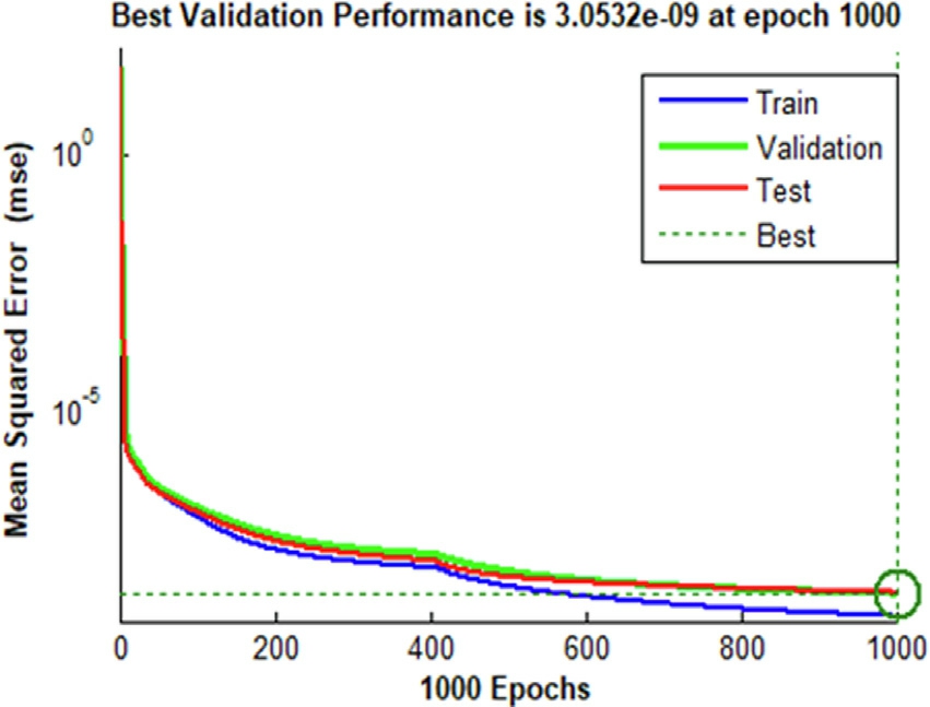
Fig.7.Performance curves of the ANN structure.
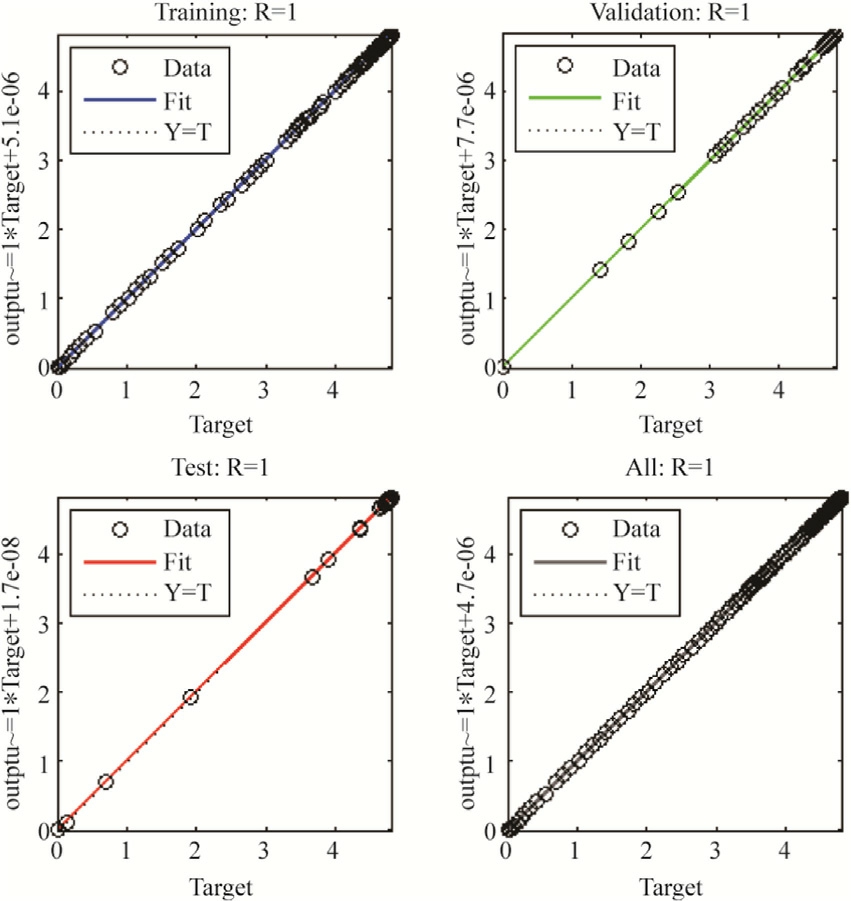
Fig.8.Regression curves of the target outputs of the implemented ANN structure.
From the second to the fourth step, the system to be monitored is subjected to only one type of disturbance ornoise at a time.The results of the residual generator for the setpoint disturbance, for the parameter noise and for the model noise are obtained respectively in Figs.10-12.Hence, Fig.10a, Fig.11a and Fig.12a clearly show that the residuals r1 are respectively sensitive to the setpoint disturbances, to the parameter noise and to the model noise.Consequently, we also note that the sensitivities of the residuals r1 in Fig.10a, Fig.11a and Fig.12a are detected via the faults fvds, fvqs and fqi respectively in Fig.10b,c,d, Fig.11b,c,d and Fig.12b,c,d.While, unlike the residuals r2 in Fig.10e and Fig.11e, the residual r2 inFig.12e is sensitive only to the white model noise,which respectively reflects the non-detectability of the fault fqm in Fig.10f and Fig.11f, and the detectability of the fault fqm inFig.12f.
In the fifth step, the system to be monitored receives both the setpoint disturbance and the white parameter noise, in order to obtain the simulation results in Fig.13.It emerges that the residual r1 in Fig.13a is entirely sensitive to the setpoint disturbance, which is immediately detected by the faults fvds, fvqs and fqi respectively in Fig.13b,13c and 13d.While,in Fig.13e,the residue r2 is not sensitive to the setpoint disturbance and the parameter noise, so nothing is detected by the fault fqm in Fig.13f.Furthermore, this 5th scenario also poses the problem of parameter noise detection, which is indeed present but we do not see it appear on r1 or r2.This specific case will be taken into account and treated in the considered fault classification protocol, in order to avoid abad diagnosis in a real operating case.
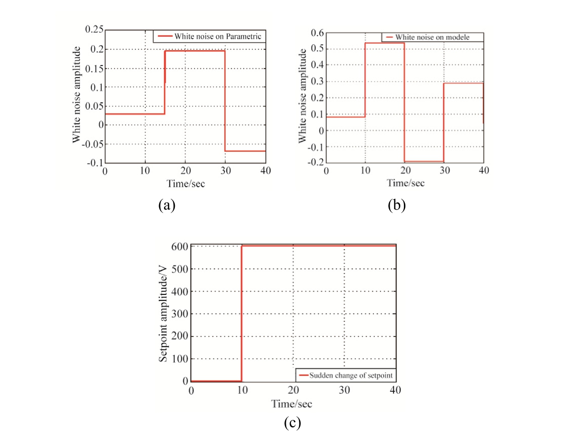
Fig.9.Representations of parameter white noise(7a),model white noise(7b) and abrupt setpoint disturbance (7c).
In the sixth step, the system to be monitored receives both the setpoint disturbance and the model noise, in order to obtain the simulation results of Fig.14.It emerges that the residue r1 in Fig.14a is only sensitive to the setpoint disturbance and directly detectable by the faults fvds,fvqs and fqi respectively in Fig.14b, 14c and 14d.Furthermore, the residual r2 in Fig.12e is also only sensitive to model noise, and directly detectable by the defect fqm in Fig.14f.Clearly in this 6th step, there is relatively no disadvantage in detecting the setpoint disturbance by r1 and indetecting model noise by r2.However, if a sensor saturation problem occurs,it is important to know that r1 will receive the influence of the model noise in addition to the strong influence of the setpoint disturbance which can obscure this model noise.
In the seventh step, the system to be monitored undergoes both parameter noise and model noise, in order to obtain the simulation results of Fig.15.It turns out that,the residual r1 of Fig.15a is entirely sensitive to model noise and very slightly sensitive to parameter noise, this isdirectly detectable by the faults fvds, fvqs and fqi respectively in Fig.15b, c and d.While, the residual r2 of Fig.15e remains only sensitive to model noise, then directly detectable by the fault fqm in Fig.15f.However,this 7th scenario poses a problem of ambiguous detection ofparameter and model noises at the same time on r1;this case will be taken into account and solved in the considered fault classification protocol.In the eighth step, the system to be monitored receives both the setpoint disturbance, the model noise and the parameter noise; however weare clearly in the scenario of the fifth step in the case ofFig.14.Furthermore, this 8th scenario still poses theproblem of fault concealment and ambiguous noise dete ction.Consequently, this scenario will be taken into account in the envisaged fault classification protocol.
Table 2 Classification of wind system faults based on DFIG.
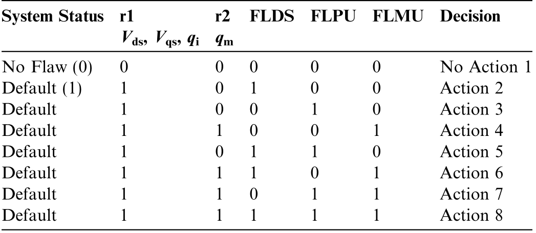
System Sta qi tus r1 Vds, Vqs,r2 qm FL LM DS FLPU F U Decision No Flaw (0 0 0 n 1 Default (1) 0 1 Default 0 0 Default 1 0 Default 0 1 Default 1 1 Default 1 0 Default 1 1) 0 0 0 No Actio 1 0 0 Action 2 1 1 0 Action 3 1 0 1 Action 4 1 1 0 Action 5 1 0 1 Action 6 1 1 1 Action 7 1 1 1 Action 8
Overall, the simulation results obtained in the previous eight steps confirm the accuracy of the fault signature table in Table 1, obtained based on the proposed robust diagnostic approach, because all the sensitivities and/or nonsensitivities of r1 have been detected or observed on the faults fvds, fvqs and fqi.The same is true when the sensitivities and/or non-sensitivities of r2 are detected or observed by the fault fqm.Furthermore, the advantage that can still be gained from this verification of the signature tableis that it offers the diagnostic system the possibility of detecting and locating a faulty sensor, because we clearly have the appearance of a fault of r1 on three sensors at the same time Vds, Vqs and Vqi.
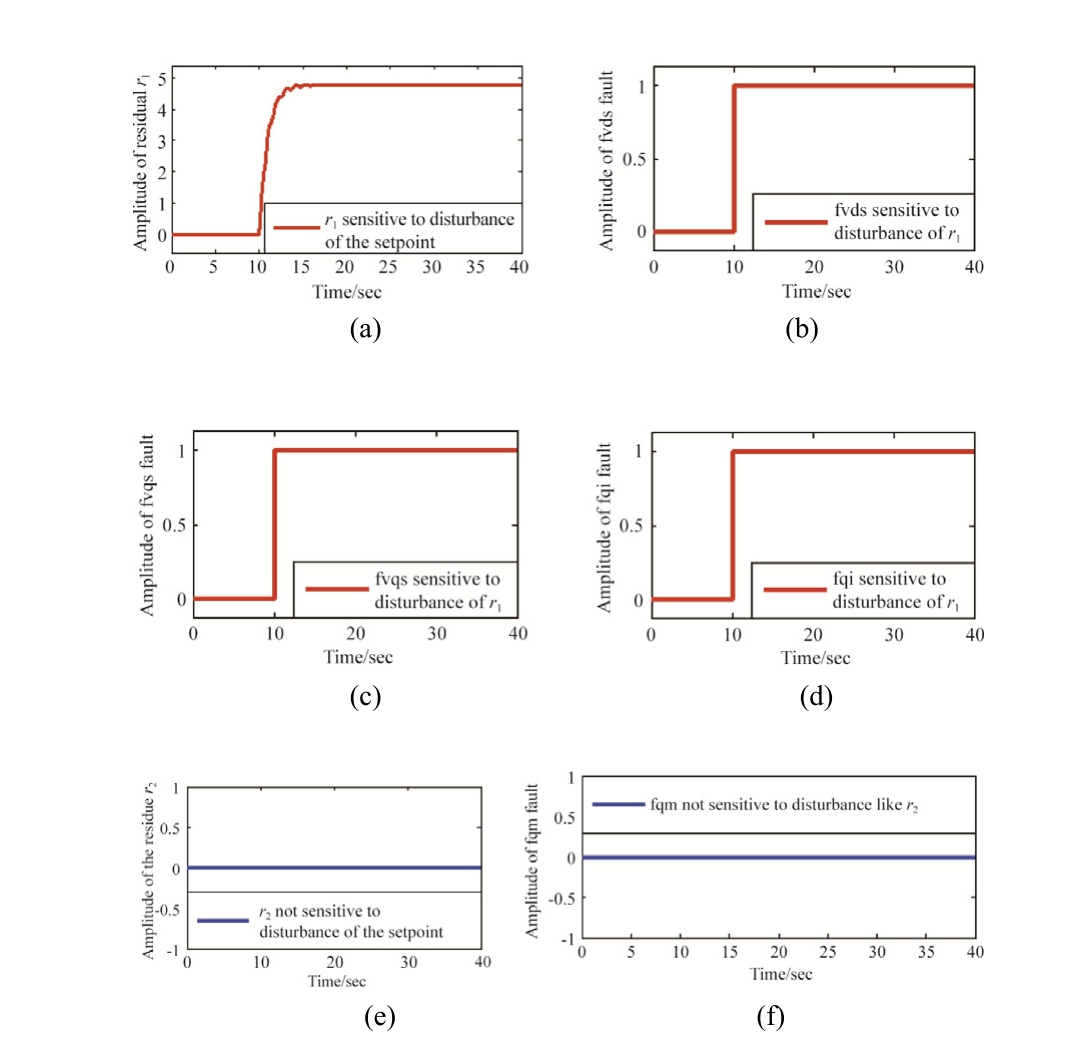
Fig.10.r1 sensitive to the setpoint disturbance(a),fvds detects r1(b),f vqs detects r1 (c), fqi detects r1 (d), r2 insensitive to the setpoint disturba nce(e), fqm observes r2 (f).
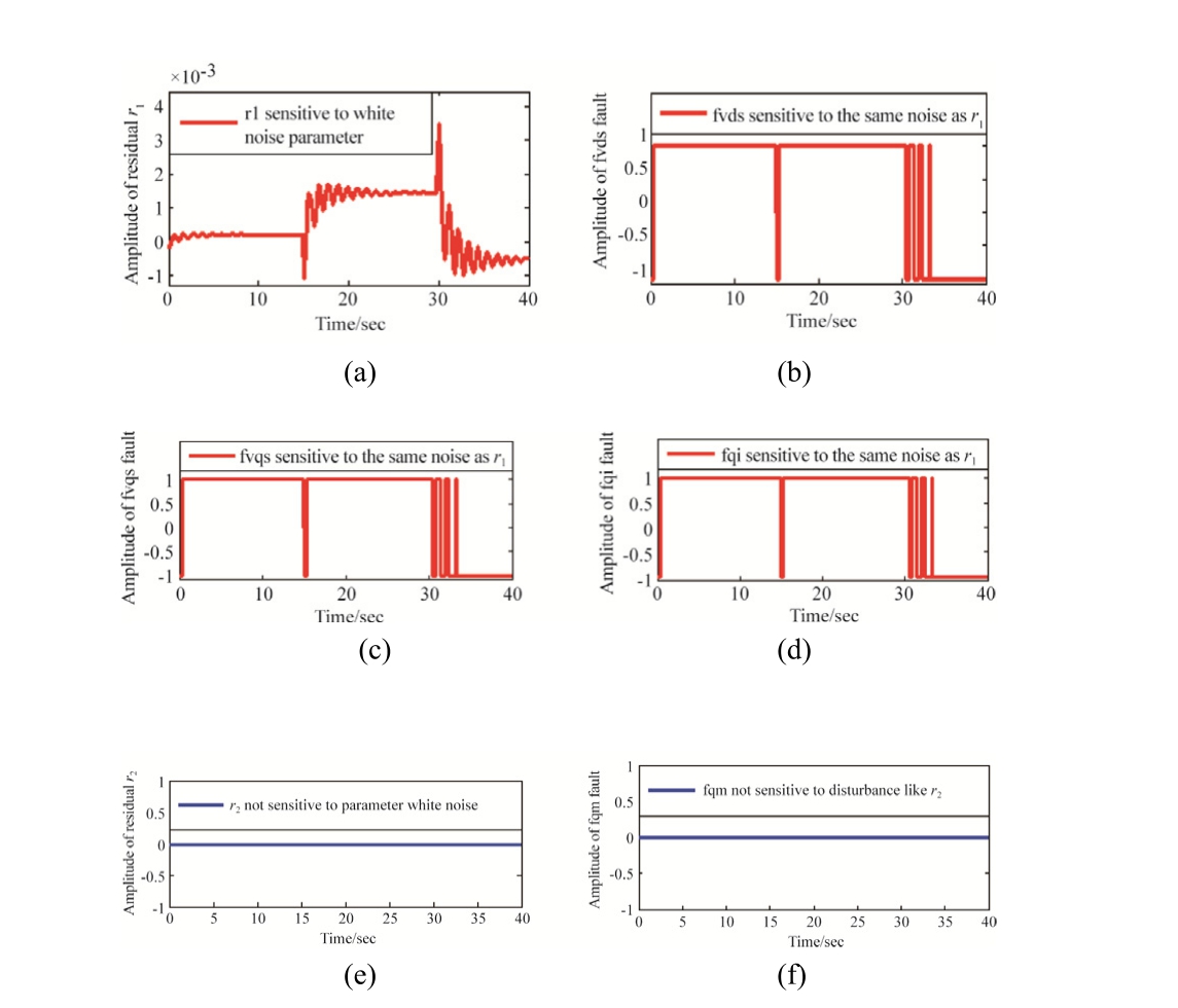
Fig.11.r1 sensitive to white noise of parameter(a),fvds detects r1(b),fvqs detects r1 (c), fqi detects r1 (d), r2 insensitive to white noise of parameter(e), fqm observes r2 (f).
2.2 Fault classification for wind system diagnosis based on DFI G
In general,we can distinguish three main types of faults in a wind power system based on DFIG,namely,the fault linked to disturbances of the setpoint (FLDS), the fault linked to model uncertainties(FLMU)and the fault linked to parameter uncertainties (FLPU) Furthermore, the causes or origins of faults are diverse in a wind power system.However,the following are the main probable causes of FLDS:
Abrupt and stochastic variations of the wind at the wind turbine;
Errors in control and adjustment of the setpoint;
The reduction in production or efficiency of the turbine.
Abnormal variations in electrical charge, etc.
In addition, the main probable causes of FLMU concern:
Modeling errors;
Degradation due to the aging of the wind energy system;
Manufacturing anomalies;
Errors during maintenance or installations (inadequate replacement of spare parts, etc.);
Whereas, the main sources of FLPU are:
Failure of the electrical integration network;
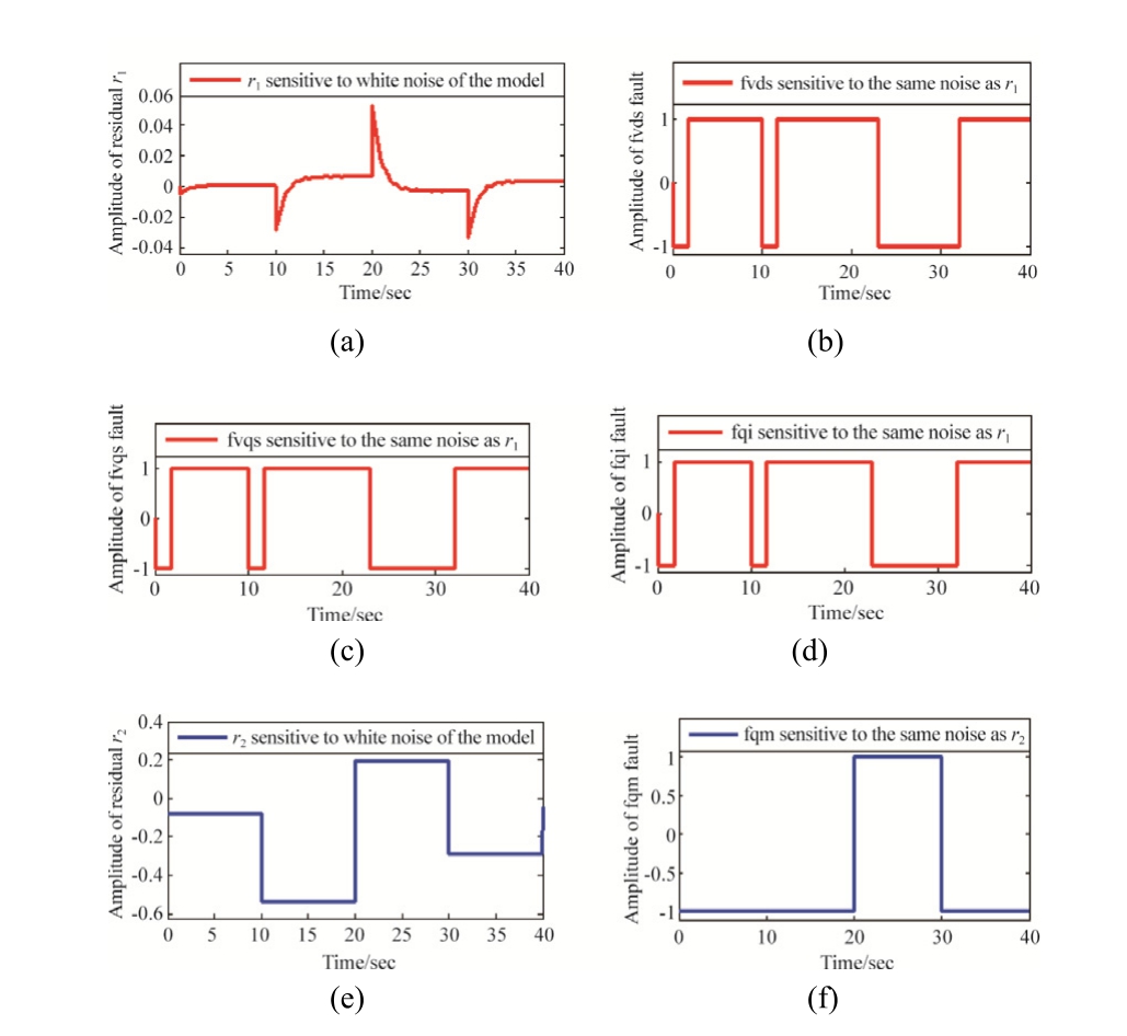
Fig.12.r1 sensitive to white noise of model (a), fvds detects r1 (b), fvqs detects r1(c), fqi detects r1 (d), r2 is sensitive to white noise of model (e),fqmobserves r2 (f).
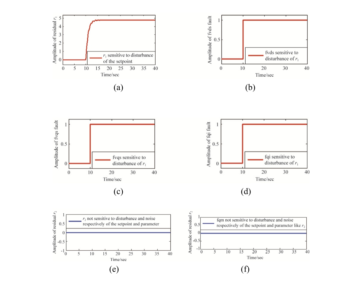
Fig.13.r1 sensitive to the setpoint disturbance(a),fvds detects r1(b),fvqs detects r1 (c), fqi detects r1 (d), r2 insensitive to the setpoint disturbance and white noise of parameter (e), fqm observes r2 (f).
Failures on the static converters of the power electronics;
Control errors;
The abnormal increase in temperature in the machine;
Magnetic induction problems between the rotor and the stator etc.
In practice, when several faults of different amplitudes occurat the same time,the system to be diagnosed is faced with two types of problems related to the detection and pr ecise localization of said faults, namely:
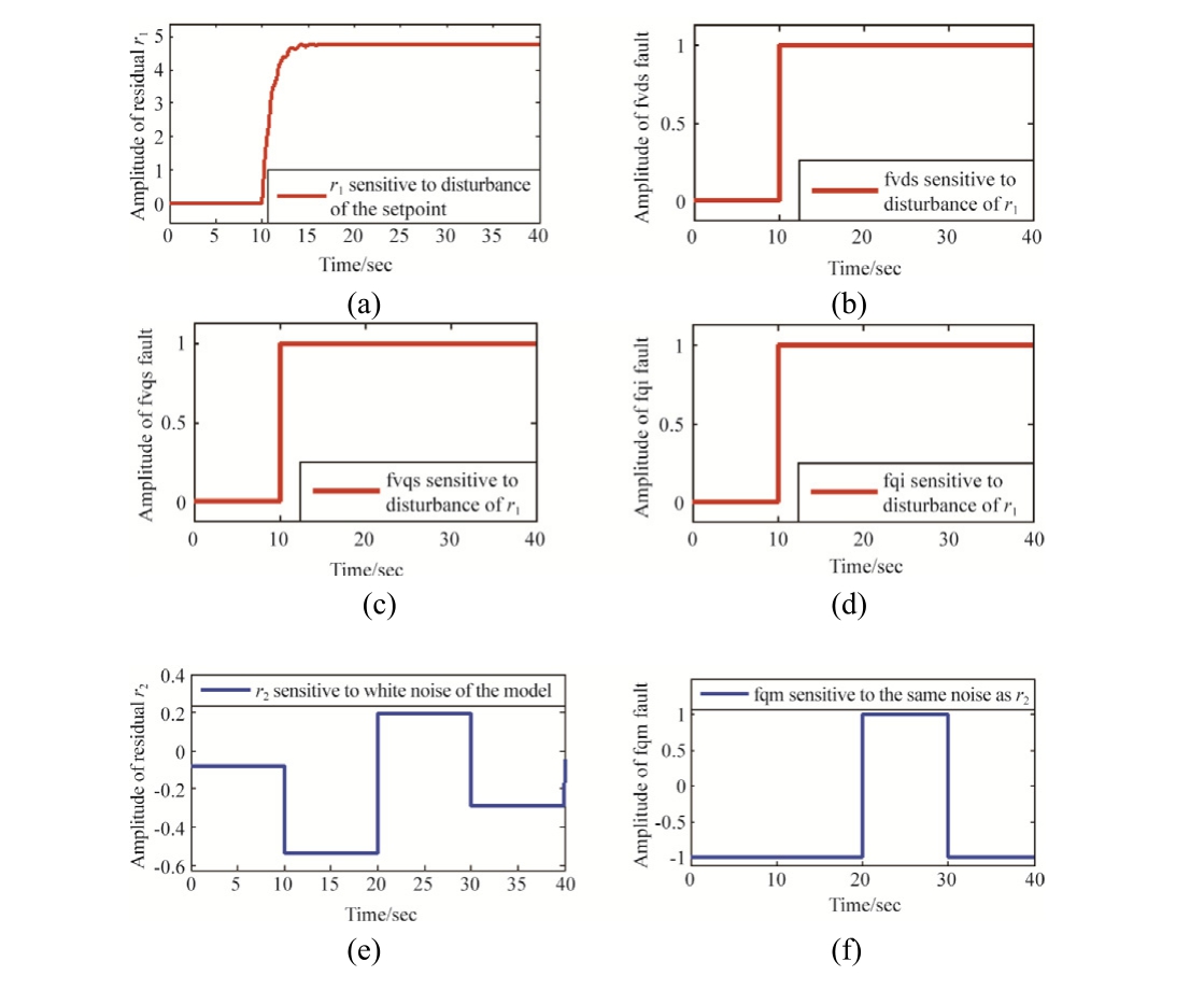
Fig.14.r1 sensitive to setpoint disturbance (a), fvds detects r1(b), fvqs detects r1 (c), fqi detects r1 (d), r2 sensitive to model white noise (e), fqm observes r2 (f).
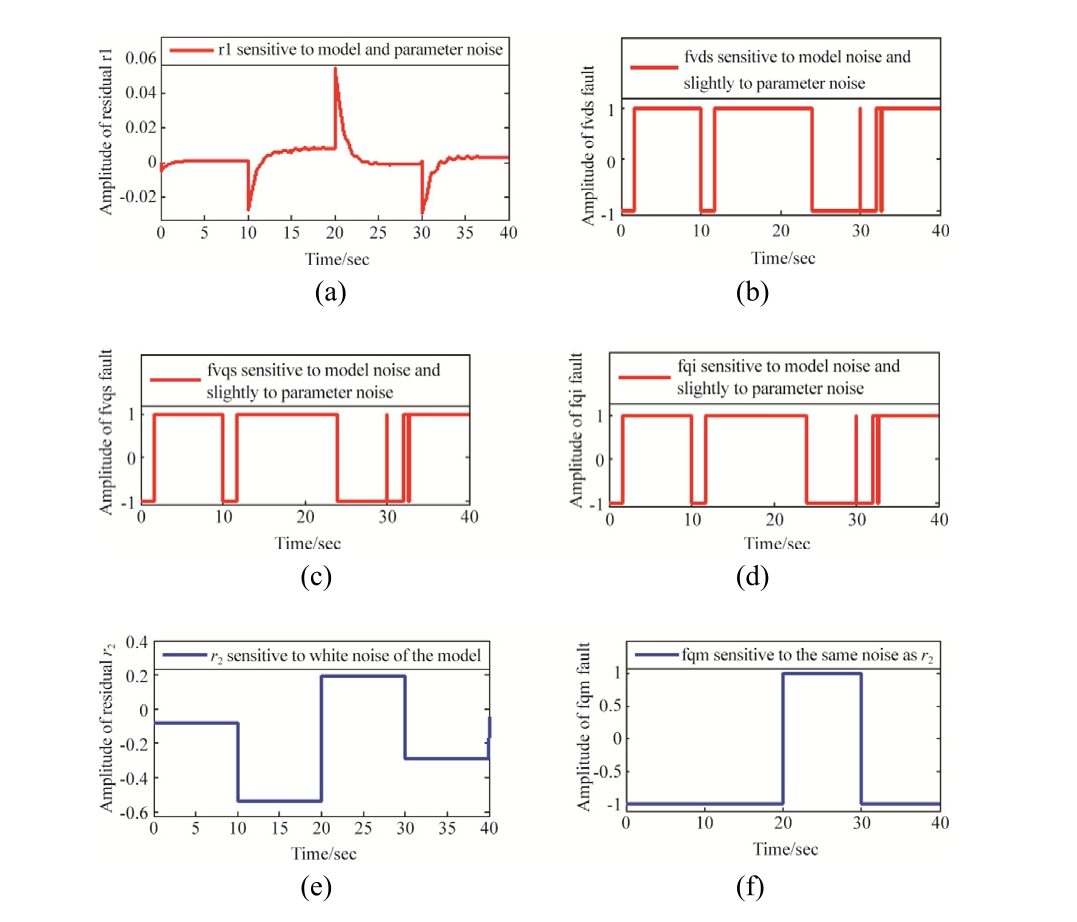
Fig.15.r1 sensitive to model white noise and slightly sensitive to parameter noise(a),fvds detects r1(b),fvqs detects r1(c),fqi detects r1(d),r2sensitive to model white noise (e), fqm observes r2 (f).
The first type of problem is when the detections of faults of higher amplitudes prevent the visualization of faults having very low amplitudes,these are the different stages observed in the cases of Fig.13abcd,14abcd, 15abcd and the eighth step.
The second type of problem which concerns ambiguous states is when the detections of faults of relatively equal amplitudes are visualized in a non-discernible way on different sensors at the same time; this is what can be observed in the cases of Fig.15abcd.
To provide effective and global solutions to the problems of detection and precise location of defects,we exploited the results of the tests and successive verifications presented in the steps of section 4.1.Accordingly,we propose a fault classification of wind power systems based on DFIG in Table 2.The latter is describedas follows:
The first column designates the state of the system to be monitored, depending on whether it is in a faultfree state or whether it is in a state in the presenceof a fault;
The second and third column are dedicated to the different possible states such as a sensitive or insensitive fault to the residues r1 and r2, associated respectively with the sensor measurements (Vds, Vqs, qi) and (qm);
The fourth to the sixth column designate the possible states of the system in the presence or absence of FLDS, FLPU and/or FLMU.
The last column represents the action decisions tobe taken in the event of a default.
The results in Figs.10-14,which correspond to the system statuses linked to actions 2, 3, 4 and 6 in Table2,clearly show that the detection, identification or precise localization of faults poses relatively no problems.However, we will nevertheless focus on the problems of detecting and localizing small defects in the cases of Figs.13-15 corresponding to the statuses of the system linked to actions 5, 6, 7 and 8 in Table 2.To do this, we will use the data from the measured outputs of the system tobe monitored to implement a classification associated with the ANN, in order to solve the problems linked to the occultation and ambiguity of detection of some of the defects reported in actions 5,6,7 and 8 in Table 2.Specifically, the main role of the proposed ANN classifier is to dedicate only one sensor to the observation, detectionor localization of the timbre or signature of a very low amplitude defect in the cases of actions 5,6,7 and 8 in Table2.This consists for the ANN-based classifier to use as inputs the measurements of the sensors Vds,Vqs,qi and qm,andto output the signature or residue r3 of the low amplitude defect sought,so that it is discernible,detectable and localizable at the same time as the residues r1 and r2.The results of the signatures or the residues of defects that we obtain in the cases of actions 8, 7, 6 and 5 of Table2,are respectively represented and verified in Figs.16-19.It appears that Fig.16a,16b,and 16c illustrate distinctly andrespectively the residues r1 for DLPC,r2 for DLIM and r3 for DLIP in the case of action 8 of Table 2.Clearly, to have r3,the output of the neural sensor must deliver a residue r3 which corresponds to the presence of the defects DLPC and DLIM, while the diagnostic system will observe the residues r1 and r2 which correspond to the presence of all the defects (DLPC, DLIM and DLIP).The ANN-based classifier will output r3 of the lowest defect in Fig.16c, by performing the following matrix addition and subtraction operation:
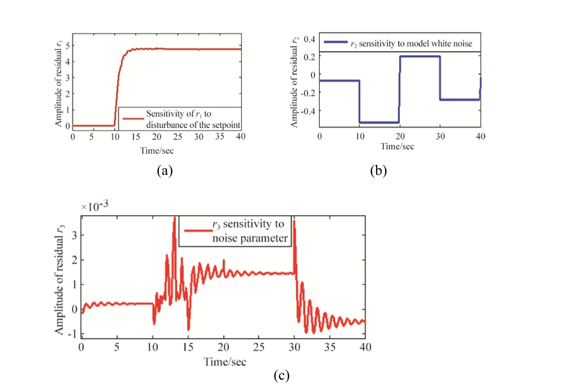
Fig.16.r1 sensitive to model and parameter noise (a), r2 sensitiveto model white noise (b) and r3 sensitive to parameter white noise (c).
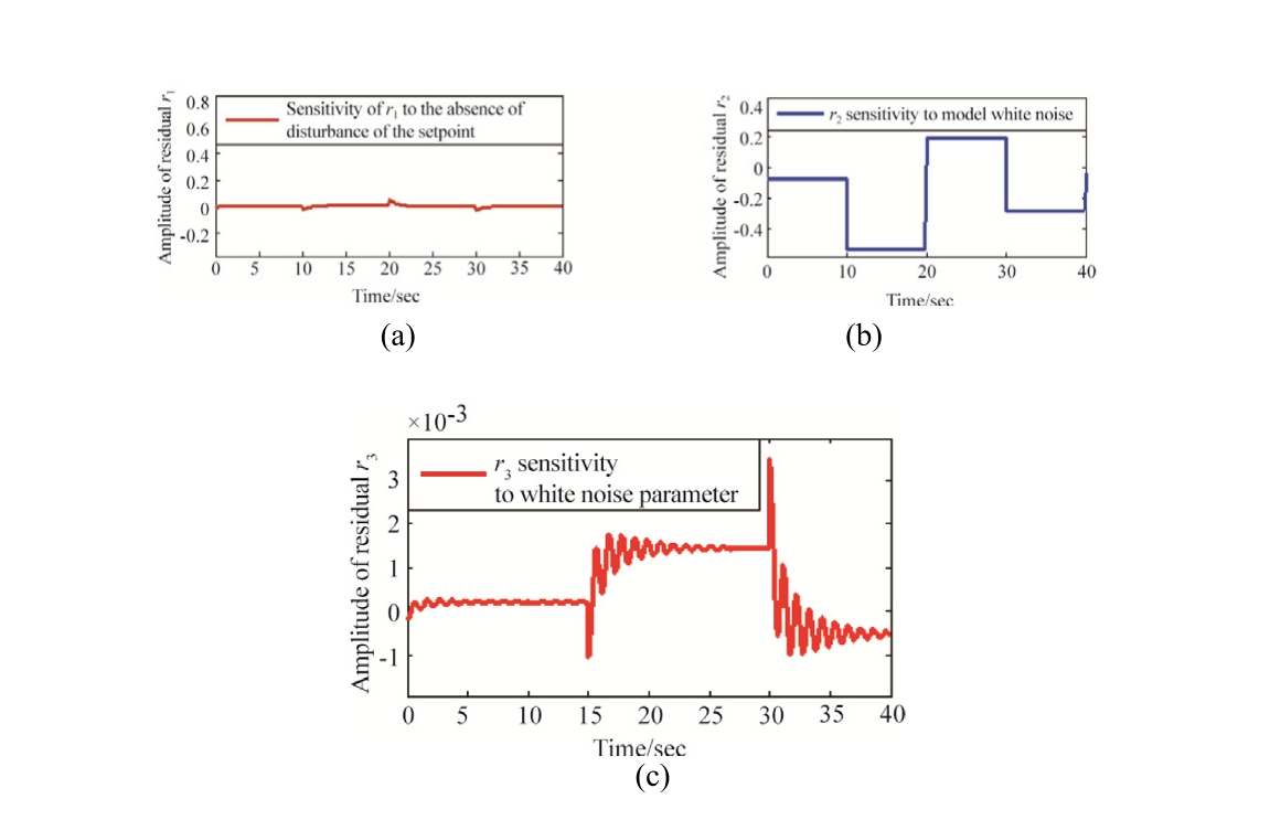
Fig.17.r1 sensitive to setpoint disturbance(a),r2 sensitive to model white noise (b) and r3 sensitive to parameter white noise (c).
When the state of action 7 in Table 2 is going to occur to the system,the classifier repeats(21),with r1 and r2 for DLIM and DLIP respectively, and r3 for (DLIM), in order to obtain the signature r3 of DLIP in Fig.17c,alongside the residues r1,r2 respectively in Fig.17a andb.
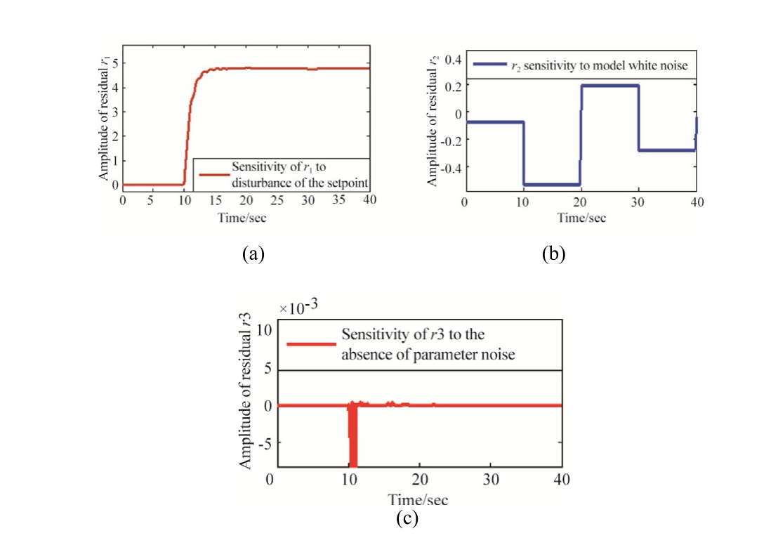
Fig.18.r1 sensitive to setpoint disturbance(a),r2 sensitive to model white noise(b)and r3 insensitive to setpoint disturbance and model white noise(c).
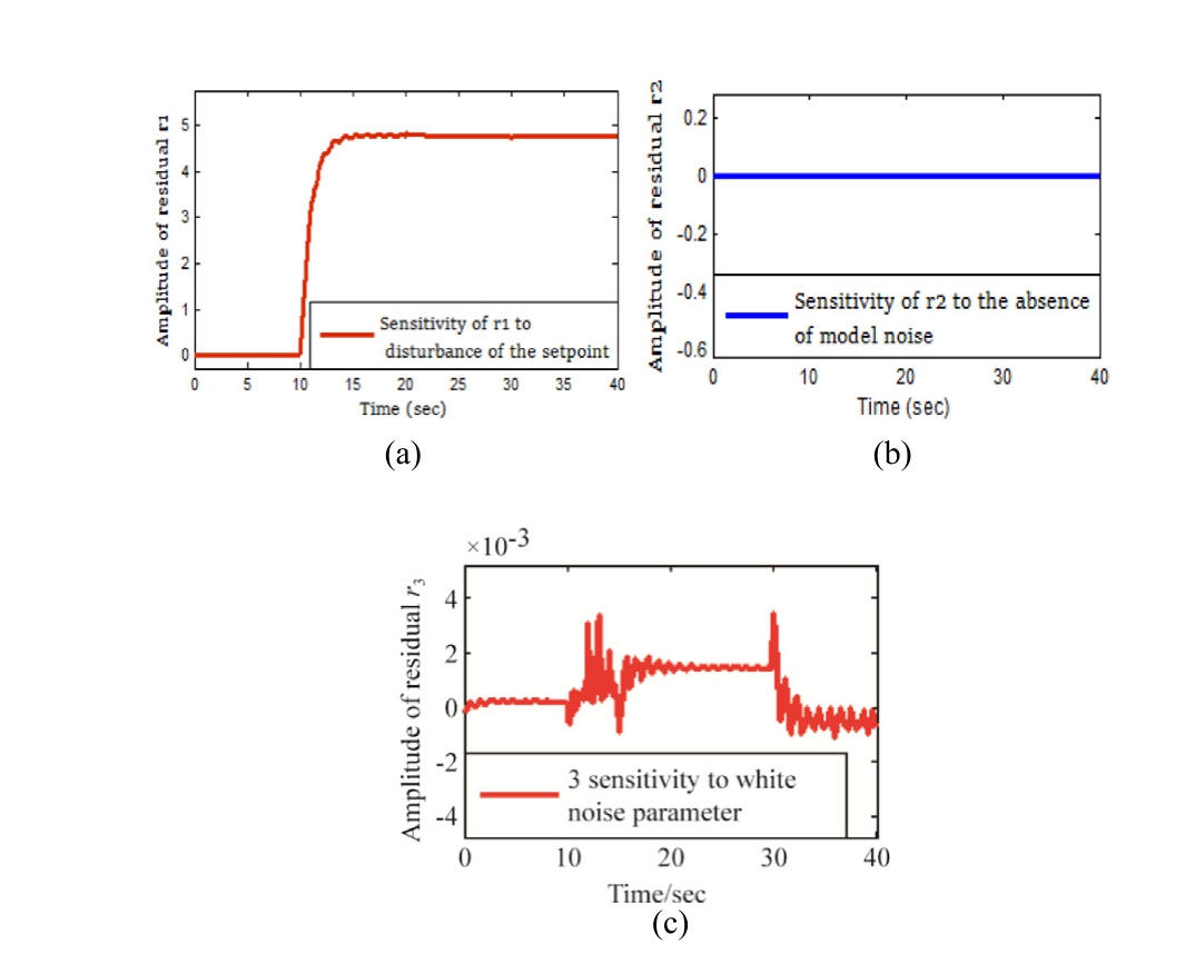
Fig.19.r1 sensitive to the setpoint disturbance (a), r2 insensitive to the setpoint disturbance and white noise of parameter (b) and r3 sensitive to white noise of parameter (c).
Then, when the state of action 6 in Table 2 is going to occur to the system to be monitored, the classification repeats the operation of(21),with r1,r2 and r3in the presence of DLPC and DLIM respectively, in order to obtain the null signature of r3 (no DLIP present) in Fig.18c,alongside the residues r1, r2 respectively in Fig.18a and 18b.Finally,when the state of action 5 of Table 2 is going tooccur in the system to be monitored, the classification repeats the operation of(21),with r1 and r2 in the presence ofDLPC and DLIP, and r3in the presence of DLPC, in order to obtain the non-zero signature of r3 (presence of DLIP) in Fig.19c, alongside the residuals r1, r2 in Fig.19a and 19b respectively.Overall, by associating the ANN with the static redundancy model, all the probable classification states of actions 1 to 8 in Table 2 have been validated, in order to clarify any ambiguity related to the occultation and/or ambiguous fault states in a robust diagnostic system proposed for wind turbines.
3Conclusion
The effective, efficient and sustainable integration of wind energy into an electrical network is fundamentally driven by the development of optimal controls and robust diagnostic strategies.Therefore,we proposed a new robust diagnostic system based on the Linear Fractional Transformation (LFT) representation combined with the static redundancy approach, in order to design a residual generator allowing the detection and localization of faults inwind power systems based on DFIG.Moreover, knowing that the faults in a wind system are of various origins,wecan nevertheless group them into three types, namely,the fault linked to the disturbances of the setpoint (FLSD orDLPC), the fault linked to the uncertainties of models(DLIM or(FLMU)and the fault linked to the uncertainties ofparameters(DLIP or FLPU).Therefore,on the basis of the results of the residual generator, it was proposed to associate an ANN with the classification in order to allow the detection and the localization of the hidden and/or ambiguous faults.It emerges that,the robust diagnostic system proposed for the optimal integration of wind turbines into the network, offers a very good compromise in terms ofreduction of complexity, economic profitability, operational safety, efficiency, security and durability of wind installations.Clearly, the proposed diagnosis allows: the use of a reduced number of sensors;the detection,the localization and the classification of faults of the wind system based on the DFIG.As well as,the detection and localization of a faulty sensor;the efficient resolution of problems related to hidden and/or ambiguous fault identifications.Inperspective, we envisage an experimental implementation of the robust diagnostic system proposed in this article.
CRediT authorship contribution statement
Boaz Wadawa: Writing - original draft, Validation,Resources,Methodology,Formal analysis,Conceptualization.Joseph Yves Effa:Validation,Supervision,Methodology, Formal analysis.
Declaration of competing interest
The authors declare that they have no known competing financial interests or personal relationships that could have appeared to influence the work reported in this paper.
Appendix A
Table A1 DFIG and PI controller simulation parameters [25].

Models DFIG PI Paramet U = 600 V/F = 50 Hz K = 0.198 R = 1.69 m K = 3.05 L = 2.95 mH /ms = 0.5 R = 1.52 m L = 2.97 mH/L /M = 2.91mH ers s p 91 s Ω i s τ r Ω r m
References
-
[1]
B.Wadawa, Y.Errami, A.Obbadi, et al., Robustification of the H controller combined with fuzzy logic and PI&PID-Fd for hybrid control of wind energy conversion system connected to the power grid based on DFIG, Energy Rep.7 (2021) 7539-7571. [百度学术]
-
[2]
A.M.Graczyk,Sustainable Energy-Defniitions,Scope,and Areas.Education Excellence and Innovation Management.Available Online: https://wir.ue.wroc.pl/info/article/WUT21b73bdb14d94a35a6ffb2c986f6fdcf/. [百度学术]
-
[3]
Q.Chen, L.Wang, S.Z.Xie, et al., Multi-dimensional evaluation and diagnostic methods for wind turbine power generation performance based on different influencing factors, IET Renew.Power Gener.18 (2024) 4249-4264. [百度学术]
-
[4]
H.Shao,R.Henriques,H.Morais,et al.,Power quality monitoring in electric grid integrating offshore wind energy: a review, Renew.Sustain.Energy Rev.191 (2024) 114094. [百度学术]
-
[5]
A.D.Bebars, A.A.Eladl, G.M.Abdulsalam, et al., Internal electrical fault detection techniques in DFIG-based wind turbines:a review,Prot.Control Mod.Power Syst.7(1)(2022)18. [百度学术]
-
[6]
M.A.Yahiaoui, M.Kinnaert, J.Gyselinck, Augmented-stateobserver-based diagnostics of open-circuit and sensor faultsin DFIG wind turbines, IEEE Trans.Power Electron.38 (12) (2023)16085-16099. [百度学术]
-
[7]
Y.Sayahi, M.Allouche, M.Ghamgui, et al., Contribution to the sensors faults diagnosis of a variable speed wind turbine:multimodel approach, in: Proceedings of 2023 IEEE 11th International Conference on Systems and Control (ICSC), IEEE,Sousse, Tunisia, 2023, pp.427-432. [百度学术]
-
[8]
W.Ding, Y.L.Jin, X.J.Wu, et al., High-resistance connection diagnosis of doubly fed induction generators, Energies 16 (22)(2023) 7516. [百度学术]
-
[9]
I.Idrissi,R.El Bachtiri,H.Chafouk,A bank of Kalman filters for current sensors faults detection and isolation of DFIG for wind turbine, in: Proceedings of 2017 International Renewable and Sustainable Energy Conference (IRSEC)., IEEE, Tangier,Morocco, 2017, pp.1-6. [百度学术]
-
[10]
I.Aissaoui, N.Elmouhi, A.Essadki, et al., Fault tolerant control for DFIG wind turbine controlled by ADRC and optimizedby genetic algorithm,Int.J.Power Electron.Drive Syst.(IJPEDS)14(3) (2023) 1382. [百度学术]
-
[11]
H.Bouazza, M.L.Bendaas, T.Allaoui, et al., Applicationof artificial intelligence to wind power generation: modelling, control and fault detection,Int.J.Intell.Syst.Technol.Appl.19(3)(2020)280. [百度学术]
-
[12]
N.Labed, I.Attoui, S.Makhloufi, et al., PSO based fractional order PI controller and ANFIS algorithm for wind turbine system control and diagnosis,J.Electric.Eng.Technol.18(3)(2023)2457-2468. [百度学术]
-
[13]
E.J.Pe´rez-Pe´rez, V.Puig, F.R.Lo´pez-Estrada, et al., Fault detection and isolation in wind turbines based on neuro-fuzzy qLPV zonotopic observers, Mech.Syst.Sig.Process.191 (2023)110183. [百度学术]
-
[14]
E.J.Pe´rez-Pe´rez, V.Puig, F.R.Lo´pez-Estrada, et al., Robust fault diagnosis of wind turbines based on MANFIS and zonotopic observers, Expert Syst.Appl.235 (2024) 121095. [百度学术]
-
[15]
E.J.Pe´rez-Pe´rez, F.R.Lo´pez-Estrada, V.Puig, et al., Fault diagnosis in wind turbines based on ANFIS and Takagi-Sugeno interval observers, Expert Syst.Appl.206 (2022) 117698. [百度学术]
-
[16]
S.Biswas, B.K.Panigrahi, P.K.Nayak, et al., A single-pole filterassisted improved protection scheme for the TCSC-compensated transmission line connecting large-scale wind farms, IEEEJ.Emerg.Selected Topics Ind.Electron.5 (2) (2024) 346-358. [百度学术]
-
[17]
S.Biswas, P.K.Nayak, B.K.Panigrahi, et al., An intelligent fault detection and classification technique based on variational mode decomposition-CNNfortransmissionlines installed withUPFC and wind farm, Electr.Pow.Syst.Res.223 (2023) 109526. [百度学术]
-
[18]
S.Biswas, P.K.Nayak, A new approach for protecting TCSC compensatedtransmissionlines connected to DFIG-based wind farm,IEEETrans.Ind.Inf.17 (8)(2020) 5282-5291. [百度学术]
-
[19]
S.Biswas, P.K.Nayak, G.Pradhan, A dual-time transform assisted intelligent relaying scheme for the STATCOMcompensated transmission line connecting wind farm, IEEE Syst.J.16 (2) (2021) 2160-2171. [百度学术]
-
[20]
M.Nazih, De´tection et localisation des de´fauts dans les convertisseurs statiques, in: Proceedings of 6TH International Conference on Electromechanical and Power Systems, 2007, pp.313-318. [百度学术]
-
[21]
V.Puig, S.Simani, Diagnostic et commande a` tole´rance de fautes 1:Techniques de diagnostic base´es sur des donne´es et des mode`les.ISTE Group, 2024.Available online https://www.istegroup.com/wp-content/uploads/2019/11/058_Diagnostic-et-commande-atolerance-de-fautes-1_introduction.pdf. [百度学术]
-
[22]
Y.J.Park, S.S.Fan, C.Y.Hsu, A review on fault detection and process diagnostics in industrial processes, Processes 8 (9) (2020)1123. [百度学术]
-
[23]
Z.H.Wang, Y.Shen, Model-Based Fault Diagnosis: Methods for State-Space Systems, Springer Nature, 2022. [百度学术]
-
[24]
W.Hwang, K.Han, K.Huh, Fault detection and diagnosis of the electromechanical brake based on observer and parity space,Int.J.Automot.Technol.13 (5) (2012) 845-851. [百度学术]
-
[25]
B.Wadawa, Y.Errami, A.Obbadi, et al., Modeling and comparative application of fuzzy logic and artificial neural network in the systemic control of a wind turbine using DFIG,in: Recent Advances in Fuzzy Sets Theory, Fractional Calculus,Dynamic Systems and Optimization, Springer International Publishing, Cham, 2023, pp.112-137. [百度学术]
-
[26]
A.Yadav,Y.Dash,An overview of transmission line protectionby artificial neural network: Fault detection, fault classification, fault location, and fault direction discrimination, Adv.Artif.Neural Syst.1 (2014) 230382. [百度学术]
Fund Information

